
All too often schedule risk analysis is perceived as an advanced and time consuming technique performed in a cursory manner only to satisfy contract bid requirements. This article shows how even simple generic analysis can highlight areas for estimate refinement and then how tools like historical analysis and estimate confidence assessments can dramatically improve the realism and achievability of schedules.
Uncertainty
Every project is subject to uncertainty. It might be simple estimate uncertainty (we don’t know exactly how long a task will take) or more complicated threats and opportunities (often collectively known as risks) that may alter the planned progression of work.
Yet even a small amount of estimate uncertainty can render a model created using the traditional critical path methodology (CPM) unrealistic. In fact, it can be easily demonstrated that anything but the most trivial CPM model will produce results that are overly optimistic and unachievable due to merge bias (a topic to be further discussed in this article). This is true even if estimates are good, execution is in line with estimates, and any uncertainty is just as likely to be beneficial as detrimental.
To learn more about this topic, watch John Owen’s free MPUG webinar on-demand, “Understanding and Managing Uncertainty in Schedules“.
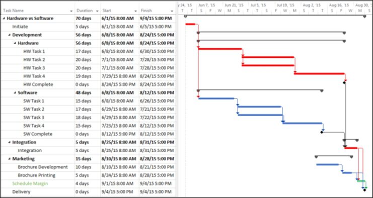
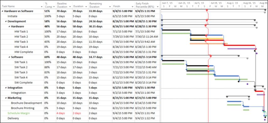
Consider the schedule shown in Figure 1.
Figure 1
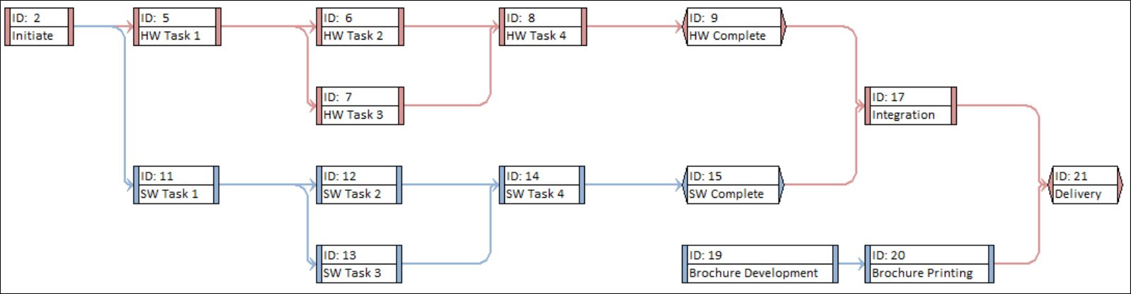
The project is planned to start on June 1, 2015. A CPM model of the schedule shows the critical path running through Initiate (ID 2), HW (ID 5, 6/7, 8) and Integration (ID17) and predicts project completion on September 4, 2015.
So, assuming that our estimates are good, how realistic or achievable is the September 4, 2015 delivery?
We know that all execution is subject to some uncertainty, but let’s be generous and further assume that individual tasks are just as likely to finish early as late. This means that each task, on average, has a 50/50 chance of being completed in the estimated duration. One might assume that this means the final project delivery has a 50/50 chance of occurring on the forecasted date (September 4, 2015). Unfortunately, this is not the case. We can demonstrate this using Monte Carlo simulation.
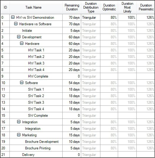
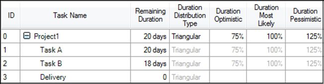
Monte Carlo is a technique that simulates the execution of a project many times. Each simulation uses a different duration for each task sampled within a range of uncertainty. This range is often called a “three-point estimate” because it comprises three estimates for each task: “optimistic,” “most likely,” and “pessimistic.” In Figure 2 you can see the uncertainty data applied to the project. Uncertainty data can either be represented as discrete durations or as percentages of the remaining duration.
Figure 2

The example reflects our assumptions that each task is subject to uncertainty and that the work is just as likely to finish up to 25 percent early as late (the most likely duration for each task has been set to 100 percent of the remaining duration).
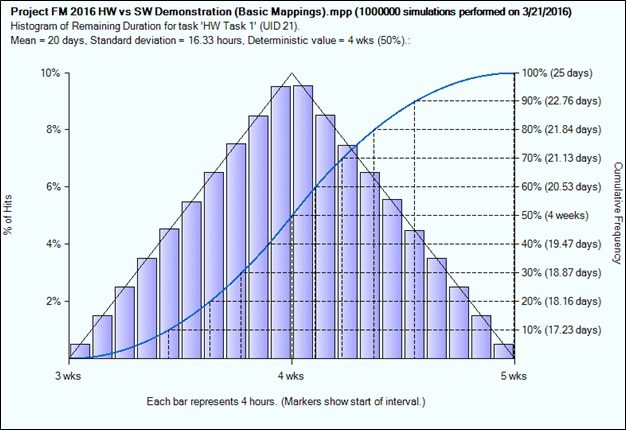
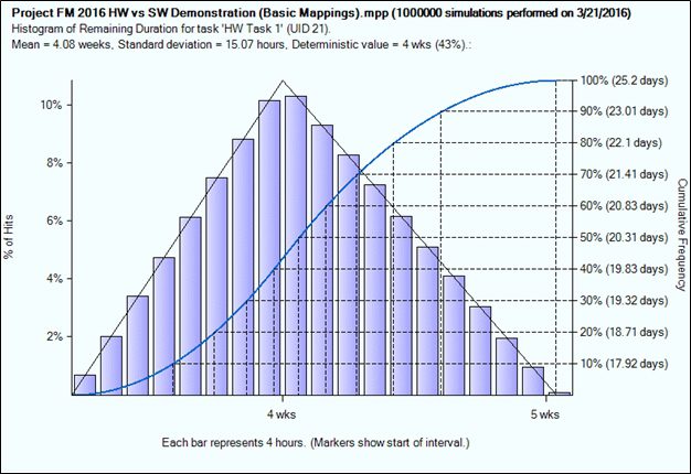
If we look at the result for a single task (Figure 3) we can clearly see that we do indeed have a 50/50 (50 percent) chance of the task finishing within the estimated duration (four weeks) and the range of possible outcomes accurately reflecting the ±25 percent range of uncertainty specified in Figure 2.
Figure 3
So if each task has a 50 percent chance of completing in the estimated duration, what is the chance of the project finishing on time?
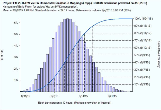
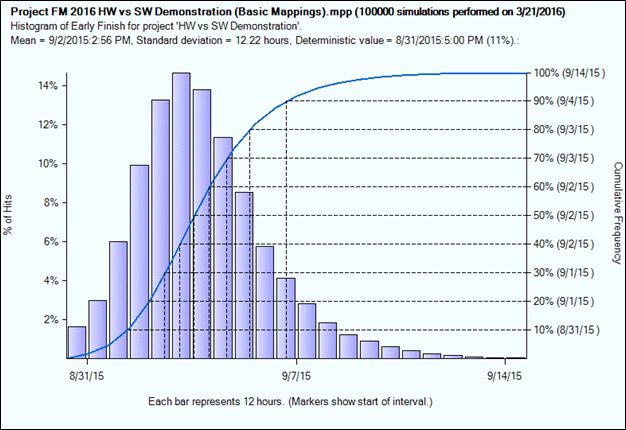
The answer is shown in Figure 4.
Figure 4
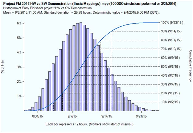
Alas, the mean (50 percent chance) finish date for the project is predicted at September 8, 2015 and the chart is predicting only a 35 percent chance of completing by September 4, 2015.
Why? The problem is that most schedules comprise multiple paths that come together (merge) in order to complete project delivery. Each merge point (a task with more than one predecessor) is an opportunity for merge bias to delay the schedule.
Understanding Merge Bias
Consider the following example where we can assume our estimates are good, uncertainty is equally likely to have a beneficial vs. detrimental impact, and historically our average actual execution time is in line with estimates.
Figure 5
![]()
If each activity takes five days to execute, the project should be completed at the end of day 10. However, what happens if Activity A takes six days to complete? As good project managers we’ll observe the overrun and focus our efforts to bring Activity B in early. If we’re successful, the project may still finish on day 10.
Now consider those same two activities executed in parallel:
Figure 6
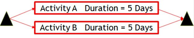
Again, each activity takes five days to execute, so the project should be done at the end of day five. However, what happens if activity A takes six days to execute? The project completion will slip to day six and there’s nothing we can do to Activity B to improve the situation. In fact, if B has any effect at all, it will only be to delay the project further.
Let’s tabulate the possible outcomes of activity A and B in our parallel example:
Figure 7
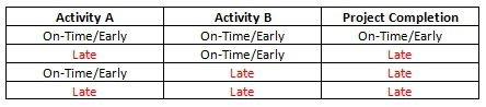
From the table we can see that, even assuming symmetrical uncertainty on the two individual activities, we only have a one in four (25 percent) chance of the project completion happening on time or early.
This phenomenon is called merge bias and is the reason why projects scheduled using CPM are inherently optimistic and produce forecast project completion dates that are often unrealistic and unachievable. Put simply, as the number of predecessors for any given task increases, it becomes less likely that it will start on time.
More Realistic Assessments of Uncertainty
In the preceding examples some quite unrealistic assumptions were used. We assumed that execution was on average in line with estimates and that any uncertainty was just as likely to have a beneficial as detrimental result.
However an analysis of past performance on similar projects might show uncertainty has a more skewed effect, as demonstrated in this figure.
Figure 8
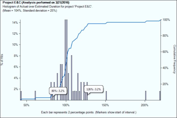
Figure 8 shows an analysis of past performance (actual over estimated duration) for a completed project. By using historical information, we can see the majority of results show a distribution that ranges from 80 percent through 126 percent with a satisfactory majority of tasks actually being completed in their estimated time (the peak at 100 percent). The outlying results (below 80 percent and over 150 percent), which we have chosen to ignore, may be due to data entry errors, very short duration tasks having a disproportionate effect, or perhaps risk/opportunities that were not identified or outlined in the schedule.
If we are scheduling a similar project, we could base our future uncertainty data on these results as shown in Figure 9.
Figure 9
Unluckily, using this revised uncertainty data, the chance of delivering the project on September 4 drops to just 20 percent as shown in Figure 10.
Figure 10
The chance of delivering on September 4 has decreased again because the chance of finishing each individual task on its estimated duration has been reduced to 43 percent (shown in Figure 11) because of the revised uncertainty data (which we derived from available historical information). On an individual task in our schedule the predicted delay isn’t large; but cumulatively and taking into account merge bias, the mean project finish has slipped another day (Figure 10).
Figure 11
If no historical information is available for similar types of projects, then other methods can be used to refine our estimates of uncertainty.
Obviously, we could request three-point estimates for each task, but this could take considerable extra effort to obtain and enter into the Monte Carlo model.
One simple first step is to try to identify tasks that are likely to matter. In a traditional CPM model one of the key outputs is the critical path. This identifies those tasks that are on the longest path through the schedule and are directly affecting the project delivery date. We could obtain more detailed three-point estimates for just these critical path tasks. However, if we remember our assumption that all tasks are subject to some uncertainty, then it becomes possible that during the simulations different tasks may become critical and affect the delivery date. Consider Figure 12.
Figure 12
![]()
Clearly Task A is driving the project delivery on 6/26 and represents the critical path. Traditionally managers focus more effort on tasks that are on the critical path; but what happens if we apply our ±25 percent uncertainty to this schedule as shown in Figure 13?
Figure 13
In Figure 14, the Critical column shows the critical path calculated by the standard CPM algorithm while the Percent Critical column shows the percentage of time each task was on the critical path after taking into account uncertainty.
Figure 14
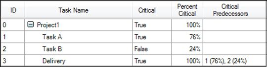
This example shows that (based on our estimate of uncertainty) Task B is driving the project delivery nearly a quarter of the time. This is important information for a couple of reasons:
We can justify the effort to obtain a more thorough three-point estimate for both tasks A and B since there is some likelihood that both tasks may affect the project outcome.
When the project is executed we should not ignore Task B from a management effort perspective just because the CPM model showed it as not affecting the project outcome. Due to the effect of uncertainty it may well affect the outcome.
So, based on our generic uncertainty we can start to identify tasks that may affect the outcome using the “Percent Critical” data from the Monte Carlo simulation. A second option is to use sensitivity analysis to analyze the impact of task uncertainty on the project delivery. Figure 15 shows an analysis of the effect of each task on project outcome for our sample project again using our generic ±25 percent uncertainty on each task.
Figure 15
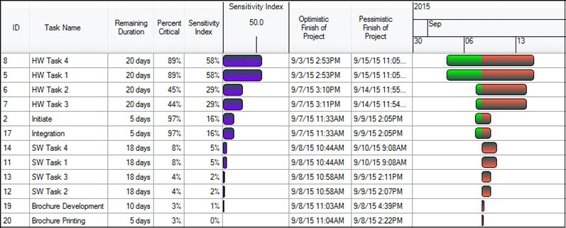
As we might expect, the project outcome has the greatest sensitivity to uncertainty on the HW (Hardware) tasks, the same ones driving the critical path in the CPM analysis. However we can also see that Initiate, Integration, the SW tasks, and Brochure tasks do have some chance of affecting the outcome (with our generic assumptions and uncertainty).
We can make some immediate decisions based on this chart. First, we’re unlikely to allow the brochure to affect project delivery, so we can decide to start that work earlier and avoid that possibility. Second, the Initiate task is largely a formality, so we probably don’t need to concern ourselves with uncertainty on that task. What is clear is that it would be worth the effort to verify and refine the estimates for all the HW and SW tasks.
As mentioned earlier, we could refine the estimates by requesting three-point estimates for each of the relevant tasks; however, this can be time consuming. One technique that can expedite the process is to review the estimates in a workshop-style meeting where the objective is not to obtain discrete three-point estimates but more simply to gauge confidence in the original estimated durations.
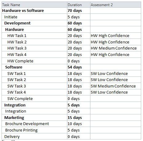
This assessment can be captured using pre-defined assessment matrices as shown in Figure 16.
Figure 16
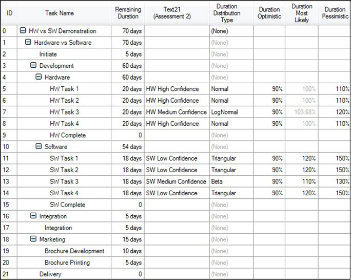
These assessments can be converted into uncertainty data for analysis by applying uncertainty templates for each assessment as shown in Figure 17.
Figure 17
The resulting analysis of project Delivery is shown in Figure 18.
Figure 18
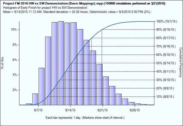
Because the assessment clearly identified a lack of confidence in the estimates for the SW tasks, a higher degree of uncertainty was applied to these tasks with the result that the chance of achieving the planned delivery of September 4, 2015 has now dropped to just 2 percent.
Achieving a Level of Confidence
Figure 18 shows a mean finish date for the project of September 14. The software is predicting a 50 percent chance of being able to deliver by that date. That also means we have a 50 percent chance of failing to deliver by that date. Most organizations don’t wish to commit to a delivery date where there is a 50 percent chance of incurring late penalties! A more prudent organization might commit to a date for which they had, say, a 90 percent confidence they could achieve.
On Figure 18, the right hand Y axis provides cumulative confidence information. Using this axis we can see that, assuming we wanted that 90 percent chance, then we should commit to a date of September 18.
But We Already Committed to September 4…
One common issue is that the required by date is beyond our control. Maybe we’ve already committed to the delivery date forecast by the CPM model or our client or other external factors control the date.
The unpalatable fact is that in order to have an acceptable chance of success (better than 50 percent), the delivery date forecast by the basic CPM model has to be earlier than the required by date.
If, as in our example, the required delivery date is September 4 and we want a 90 percent chance of achieving that date, we’re going to have to adjust the underlying CPM model to bring the end date forward — earlier than the required by date of September 4 — with the aim of the subsequent risk analysis showing a 90 percent confidence for September 4.
The Percent Critical and Sensitivity Analysis can help identify opportunities for schedule compression.
Figure 19
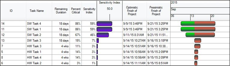
In Figure 19 we can see that uncertainty on SW Task 4, SW Task 1 and SW Task 2 is having the greatest effect on the delivery outcome and that when these tasks finish early, then the project also tends to finish early. So these are good opportunities for review. Perhaps we can reduce uncertainty by using more experienced developers or reduce the duration by applying more resources.
After making the changes to SW Task 4, 1, and 2 duration and estimate confidence values shown in Figure 20, our chance of delivery on September 4 rises to 20 percent. The revised sensitivity analysis is shown in Figure 21.
Figure 20
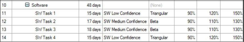
Figure 21
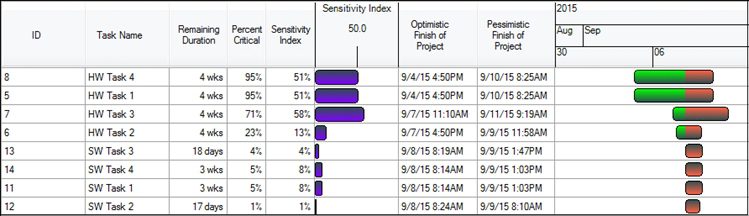
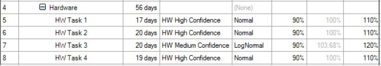
We can see that HW Tasks 4 and 1 are now driving the schedule (95 percent critical) and early finishes for these tasks tend to make the project finish earlier. In Figure 22 the durations for HW Tasks 1 and 4 have been modified.
Figure 22
These changes provide the result shown in Figure 23, where the 90 percent (P90) confidence date is now September 4 as required.
Figure 23
By bringing in the CPM finish date to August 31, we have increased the probability of being able to deliver on September 4 to 90 percent.
Schedule Margin
In our example, we were forced to adjust the underlying CPM model to forecast a delivery date that is earlier than the required date in order to achieve a 90 percent level of confidence in the final delivery date.
In order to clearly identify that we’re not committing to an earlier delivery on August 31, we need a placeholder to explain the difference. Such placeholders have had various names: “contingency,” “delay allowance,” “risk allowance” and “risk buffer.” More recently, various industry organizations including the Project Management Institute (PMI) and National Defense Industrial Association (NDIA) have adopted the term, “schedule margin” as the term for this place holder.
Schedule margin is defined as “the amount of additional time needed to achieve a significant event with an acceptable probability of success.”
In Figure 24, a schedule margin task of four days has been inserted before the final delivery milestone. This moves the delivery milestone out to the contract delivery date of September 4. The schedule margin is owned by the project manager.
Figure 24
As the project progresses, the actual duration of tasks will be captured and may be different to the original estimated duration. We hope it will be within the range of uncertainty specified for the task.
As the remaining duration of the project changes, the schedule margin task will expand or contract so the delivery remains on September 4. The project manager will monitor the consumption of the schedule margin to ensure the required date is achieved.
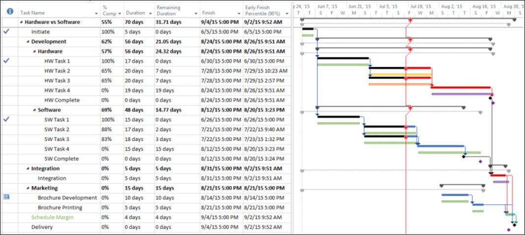
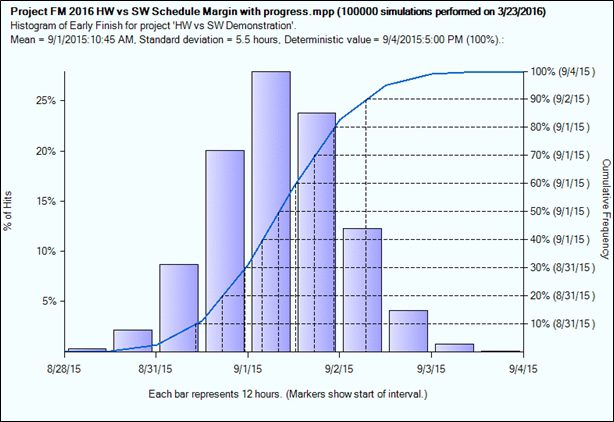
Consider the example in Figure 25. The project is just over 50 percent complete, and all work is being completed on time (based on the revised schedule after compression). The schedule margin is still four days for a delivery on September 4. However, note that the delivery “Early Finish Percentile” (90 percent) is now showing September 2 rather than September 4. In fact, if you view the histogram in Figure 26, it’s clear that the range of uncertainty for project delivery has diminished significantly. (Standard deviation for delivery is now 5.5 hours compared to 12.22 hours before the project started.) As the remaining work decreases, the remaining uncertainty also decreases.
Figure 25
![]()
Figure 26
In Figure 27 we see an example where planned progress hasn’t been achieved on the HW tasks. Fortunately, the slippage has only consumed two of our four days schedule margin (highlighted in red) and the projected Early Finish Expected (P90) is still September 4. While it might be expected that the Early Finish Expected (90 percent) would have slipped beyond September 4, in this case, despite the slippage, the reduction in remaining uncertainty (because the whole project is roughly 50 percent complete) still gives us a good chance of meeting the September 4 date. In reality, the Early Finish Expected (90 percent) has slipped compared to the September 2 date shown in Figure 25 which was based on perfect progress.
Figure 27
![]()
Understanding and managing uncertainty in schedules dramatically improves the chances of project success. It also reduces surprises, which in turn reduces management effort and cost.